There have been numerous projects (Zuo 2007, Chronis 2010, Karagkouni 2012, Shelby 2011) using FFD simulation environment based on initial Stam paper 1999. A detailed explanation of mathematics and algorithms behind the solver can be found in Chronis 2010 and it is out of scope of this thesis to extensively explain details of Fluid Solver implementation. Instead, a basic explanation of important design aspects of the solver is presented to assist the reader in following up the context of the thesis.
The basic algorithms explained in 2D environment by Stam 1999 were ported into 3D by Ash 2006 and later on implemented in processing.js by Chronis 2010. The only variation to the initial implementation on processing.js in current thesis, is the addition of Vorticity Confinement force to help with Stam’s “numerical dissipation” issue as explained by Fedkiw 2001. This extra force is explained in detail by Shelby 2011 and the reader is encouraged to use it as a reference to gain deeper understanding on the matter.
Returning to the actual Fluid Solver implementation, the basis the solver is built upon, are the Navier – Stokes equations which are used to describe physical fluid flows. These equations are really hard to solve so Stam’s effort is to produce a stable and fast algorithm that could be advanced in discrete steps by compromising physical accuracy the precise mathematical models would give. The equations governing the flow movement are shown below:
From Mathematics point of view, the state of a fluid at a given instant of time is modeled as a velocity vector field (Stam 1999). The equations above show that a change in velocity occurs depending on three different terms. The diagram below (Fig_30) shows what these terms are representing. An interesting point that has to be pointed out at this stage is that velocities of the fluid would not be really visually interesting and what is actually visualized is the density of a moving object through that fluid. Density is a continuous function that takes values between [0-1] and for every point (voxel) in space tells us the amount of “particles” present. The solver is mainly following below state diagram (Fig_31):
As a final note, what is critical into the solvers success is the ability to implement a stable solver to the linear system diffusion steps inserts and this has been done using a Gauss – Seidel relaxation algorithm. Another important aspect of the solver is how internal and external boundaries are defined but this is explained in detail on the following section.

equation_1

equation_2
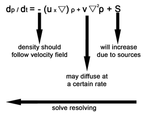
Fig_30
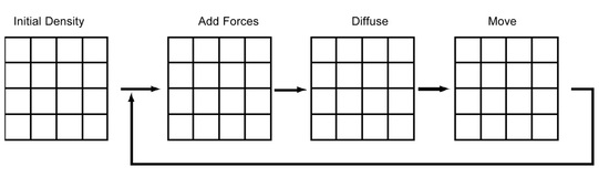
Fig_31
