Basic objective of this methodology step is to find the optimum tensegrity unit that can effectively serve the purpose of a windbreak structure. This step has been implemented with the usage of Genetic Algorithms (GA). Genetic Algorithm is a technique from the field of Evolutionary Computation developed by Chandana Paul et al. (2005) to optimize complex problems by mimicking the natural evolution process. In this section, the whole approach and implementation will be explained but in depth explanation of how genetic algorithms operate is out of this thesis scope and the reader is encouraged to read relevant literature.
Having understood the way tensegrity structure is modeled in our simulation environment, the first choice we had to make is what genes our tensegrity would have. Defining the genes is one of the most critical parts both in GA and in real life natural evolution. The genes are the essence of what we try to model/examine and should be able to construct it without further information. In our case it is believed that the minimum amount of information we need to describe a tensegrity unit is the number of joints, the length of its struts, the connectivity pattern between the joints and finally the information of which connections are struts and which are cables. Given the fact that number of joints (hence number of struts) is stable per run, what have been chosen as genes are below:
1. The length of struts.
2. The connectivity pattern.
3. The definition of type of connection.
These characteristics (genotype) define a tensegrity structure as a whole but its actual combination to one entity is what we call phenotype in GA terms, which is the essential building unit of an individual, which in turn corresponds to a single actual tensegrity. Finally what is referred as population is a collection of individuals (25 in our case) that works as the initial seed of the process. The explanation of these terms is of crucial importance for a reader to follow up the description of GA implementation. A final important GA term that must not be overlooked is what we call fitness and is actually closely related to the phenotype. The fitness is the actual optimization metric that GA are trying to get to and is the actual way of comparing the individuals between them and find the fittest of all that will survive the process. There are numerous other GA terms (evolution, mutation, etc.) but the ones mentioned here are the fundamental ones on which the simulation is built upon.
It is now time to get to the actual description of our approach. Our first step is to create an initial population of 25 individuals. What this means in essence is that for every single individual, first genes are created, then they are combined to phenotypes and this now has the info needed to define an individual. A very important step, called swap technique takes place at this point and is what is explained in detail on the paper Evolutionary Form-Finding of Tensegrity Structures by Chandana Paul et al. (2005). For every individual, during the creation of its genotype the process followed is shown in the diagram below (Fig_26). Swapping technique is a very intelligent way to create tensegrities with different connectivity patterns (hence different tensegrity units) but always ensuring that tensegrity properties are maintained. What it actually does is randomly chose 2 struts and swap their places honoring various constraints. This also visualized clearly in the diagram below (Fig_27).
At this point we have created our initial population of tensegrities and we have managed to create a variety of different tensegrity units based on the length of their struts and their connectivity pattern. It has been explicitly decided to always keep the number of struts stable per run because after various experiments it has been found that it is not fair to have tensegrities with different number of struts to compete. A good initial population in GA world is one that has as much variability as possible but at the same time all the individuals must be able to fairly compete with each other for the GA to work. Next step after the careful population creation is to let the tensegrities behave and simulate and actual form a stable structure by leaving its particles interact with each other until they reach equilibrium. This is generally referred as form finding process in tensegrity context and this is exactly what is happening at this step, is letting the tensegrity find its form and reach a stable state. A usual step implemented to help tensegrities reach an equilibrium state quicker is what is referred as dynamic relaxation in tensegrity form finding research but this has not been found necessary to be part of this thesis and could be a future enhancement. So, once we ensure that all tensegrities have reached equilibrium and are considered stable our next step is to evaluate them. This is where fitness comes into play and in our case Fast Fluid Dynamic (FFD) simulation as well. FFD details will be explained in the following section but this step can be explained in general terms. Per individual, we create a FFD simulation environment and we simulate tensegrity behavior under it as shown in image below (Fig_28). There are quite a lot of things that need to be discussed regarding this implementation but everything will be clear in the next section that explains what happens in the FFD environment. What is important at this stage is define what we consider our fitness. We try to minimize the air that passes through our tensegrity unit hence we count the mean air velocity per square meter in a specific location “behind” the tensegrity and try to minimize it. So the smaller this number is the fittest our individual is considered to be.
Once the whole population is evaluated it is then sorted based on their fitness and we are ready to start what is called evolution state in GA terms. What happens at this step is discard the 10 less fit individuals and create new ones (referred as children) mainly based on the characteristics of the fittest ones. This is the part where evolution happens and the algorithm starts working towards finding the optimum solution. The whole approach of how we create the 10 new children per generation is clearly explained in the diagram below (Fig_29). Four children are created with a single strut swap from the winner of the tournament selection process and six more are created with strut swaps of the rest of the individuals. The tournament selection is a way to fairly select a fit individual to give birth to new children. Three different individuals enter the tournament with higher chances to be close to the fittest member of the population and the winner is of the tournament is the fittest. Part of the evolution step is what we call mutation as well. This corresponds to a five per cent possibility the genes of the new child to get mutated, which actually means change radically and not based on the normal evolution process. When all children are created they are left to reach equilibrium state and then evaluated as explained above and then we move into the next generation evolution.
This procedure is repeated for 20 generations and the fittest individual of all is the optimum result we were looking for. The whole GA procedure has been run for tensegrities with different number of struts and results have been kept in all cases to give more flexibility and options when it comes down to actual tensegrity structure implementation at the final step of this methodology followed.
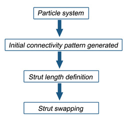
Fig_26
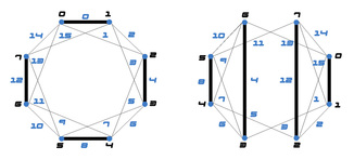
Fig_27
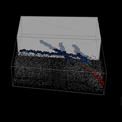
Fig_28
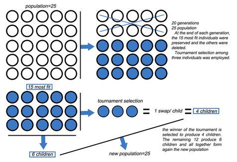
Fig_29
