In order to be able to simulate the behavior of tensegrity structures in accordance with physical world environment, they were treated as particle systems. In this context, what we mean by particle system is a collection of points in 3D space with specific masses connected with each other with elastic springs. As this is fundamental on how we approach the modeling of a tensegrity structure within our computational environment, it was deemed necessary to present a basic introduction on Particle system usage.
You can think of all tensegrity joints as the particles. The three basic characteristics needed to construct them are their initial location in 3D space, their initial velocities and their masses. In our efforts, all particles are assumed static and with minimal masses as their starting point, not to interfere with movement calculations. Next step is to connect particles with springs following a specific connectivity pattern that will be explained later on this section. All springs honor Hook’s law (Fig_23):
The point masses are connected with elastic springs where each spring has a defined rest length L0. In our case, at this step we decide (allowing some variability in the process) which spring connections will be struts and which ones will be cables. We do that, because we will define springs with different characteristics in each case. A spring, when it is displaced from its original position and its length changes it starts exercising a force trying to return to its initial rest length. The magnitude of this force depends on its displacement (x-x0) and its spring constant (k). The acceleration of a particle is given by:
Acceleration = k*displacement/mass
Having said that, it is time to explain how these fit with a tensegrity structure. The tensegrity struts are defined as very strong (high spring constant) springs and their rest length is defined to be equal to their physical length. The cables on the other hand, are defined as weak springs with rest length equal to zero. This approach helps us model the elements of the structure (Fig_24). So by defining a particle system with above properties we have almost created a tensegrity structure, but there is one thing still missing. Tensegrities have to honor very specific properties to be considered as such. Throughout the designing process the tensegrity unit properties should be maintained. The most significant properties that should be set and ensure the topological validity of the tensegrity unit are the number of the struts and the connectivity pattern that defines the connections between struts and cables. The connectivity pattern forces firstly the struts to have the same number of connection with the cables (3 or more cables per strut) and also ensures that two struts cannot share a common joint (Chandana Paul et al., 2005). These tensegrities treated here are called “Class 1” tensegrities and follow the specific properties. The initial connectivity pattern is presented in the diagram below (Fig_25). Choosing this connectivity pattern as our starting point is not a random choice and is closely connected with maintaining the tensegrity properties discussed above through the next process of Genetic Algorithms.
A final note that should be made clear at this point is that having defined the tensegrity structure, the only thing one has to do to simulate its behavior is let the particles interact with each other until the structure finds its equilibrium state. To effectively do that there are two extra points that should be taken care of. For every tensegrity particle (joint) a list of other particles that are affecting it is kept throughout the process and there has been some extra constraints implemented to assign some physical mass to the springs connecting the joints and model their possible collisions.
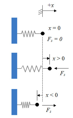
Fig_23
F= k (x- x0),
x0 = initial position
k = spring constant (elasticity)
x = current position
F= k (x- x0),
x0 = initial position
k = spring constant (elasticity)
x = current position
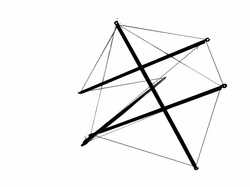
Fig_24
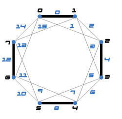
Fig_25
